A Brisk Intro to Reinforcement Learning
How do humans learn? Unlike a successful image classification pipeline, humans do not require millions of labelled examples to distinguish chairs from tables. Instead, we learn by interacting with the environment, requiring no labelled supervision at all. How is this possible, and can it be replicated on a machine?
This spring I had the privilege of attending The Recurse Center in New York City and one of the topics I was keenest to explore is reinforcement learning. Reinforcement learning algorithms teach agents by letting them interact with an environment, much like humans do. What do these algorithms look like?
Monte Carlo RL: The Racetrack
Let's get up to speed with an example: racetrack driving. We'll take the famous Formula 1 racing driver Pimi Roverlainen and transplant him onto a racetrack in gridworld.
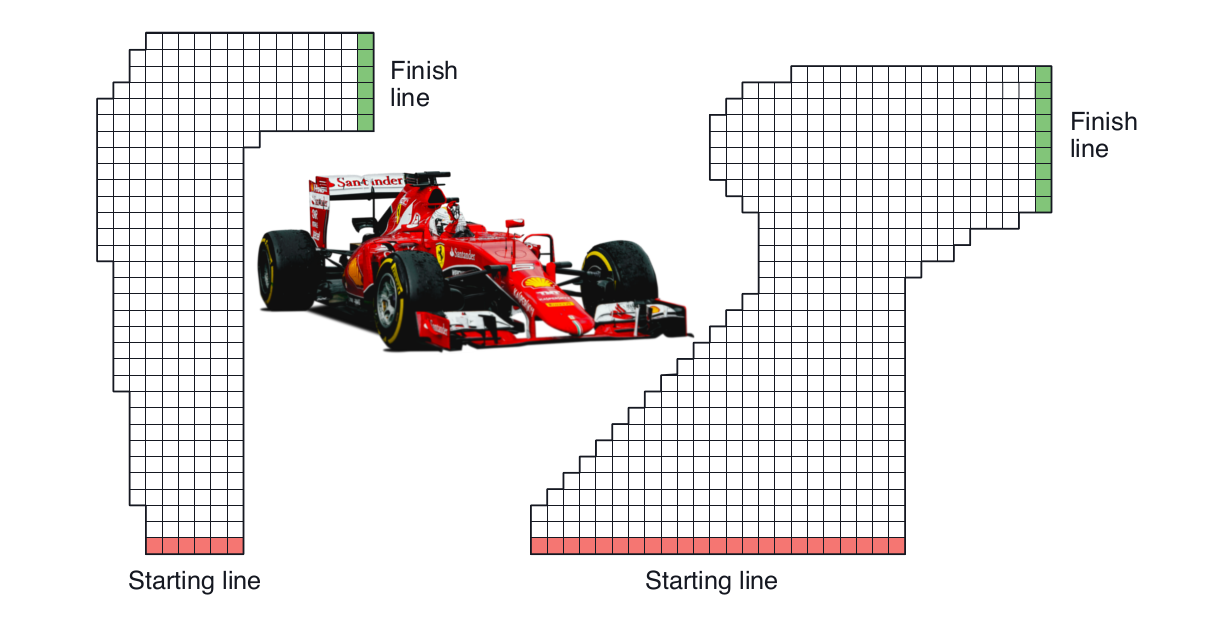
The idealised racetrack
Pimi's task is to learn how to drive from any given point on the red starting line to any point of his choice on the green finish line. He should do this as quickly as possible. We'll model Pimi's driving in a simplified way: namely as a sequence of moves from square to square. After each move he gets to accelerate by +1, 0 or -1 velocity units in either or both of the X and Y directions, giving a total of 9 possibilities(+1,+1), (+1, 0), (+1, -1), etc.. His new velocity then determines in which square he'll end up next. For safety, let's cap both the X-speed and Y-speed at 5 units.
This example is taken from the book "Reinforcement Learning" by Richard Sutton and Andrew Barto, 2018 Edition, Chapter 5.7, p111. I'll be referring to this book frequently and absolutely recommend it as an introduction to reinforcement learning.
We can write down our task using more formal terminology. Our task is to learn the best possible action in the given state we're in. In this case, a state is one of this possible cells in the grid and at each cell there's 1 of 9 possible actions we can choose from. In other words, we have to learn an ideal policy, an ideal mapping from states to actions. Again:
- states
\(S\)are defined to be the possible cells in our grid - actions
\(A\)are defined to be the 9 possible accelerations we can perform at each state - The policy is our current strategy for selecting the action given the state
we're in. This is a mapping
\( \pi: S \to A \). Pimi's goal is to learn the best possible policy.
On such an easy course, this is an easy task for Pimi. So, to make things harder,
we'll blindfold him so he cannot see where he's going. All he has access to is
9 success logbooks at each square in the racetrack -- so \(9N\) logbooks,
where \(N\) is the number of squares in the track. Each logbook belongs to 1 of
the 9 possible accelerations Pimi could make, say for example \((+1, 0)\). Then
this logbook \((+1, 0)\) has a
full record of the number of moves it's taken Pimi to
arrive at the green line in the past starting at the current square, given
that the action taken was \((+1, 0)\).
As Pimi drives with his blindfold on, he drives at random by accelerating in
random directions because he can't see where he's going. He often crashes and
when this happens, he takes a sip of refreshing blueberry juice, fetches a
plaster or two and then starts again from a random point on the red starting line,
keeping a stiff upper lip. As he does so, he crosses more and more squares, the
smoke rises, the racetrack gets worn and the \(9N\) logbooks fill up.
That's a lot of paper!
Once there's a fair amount of records in each of the \(9N\) logbooks, Pimi can
start using them to make decisions instead of driving and crashing randomly.
Each success logbook is indeed a measure of success of its corresponding action at that
square in gridworld: the logbook averaging the lowest number of moves
to completion should intuitively correspond to the best action. Why? Because
the logbooks tell us exactly which of the 9 actions has, on average, a more
desirable outcome. If for example logbook 3 corresponding to action \((+1, -1)\) averages
87 moves to completion, and logbook 2 corresponding to action \((+1, 0)\)
averages 56 moves to completion, then choosing \((+1, 0)\) is measurably
better than choosing \((+1, -1)\).
This intution is in fact correct and has solid theoretical
underpinningsSutton and Barto, Chapters 3-5.
The particular approach just outlined is an example of a class of
algorithms called Monte Carlo algorithms in reinforcement learning. These
algorithms learn the value of a particular action \(a\) taken at a state
\(s\) by running many trials and evaluating the consequence for each trial.
In our case this means letting Pimi race again and again and counting the
number of moves it takes him to complete the track each time. The final value
of action \(a\) at state \(s\) , denoted \(q(s, a)\), is then the
average length of time to completion after that action, averaged over all of
the trials. We can then use these value estimates to update our policy, our
strategy for selecting actions. Pimi takes his logbooks, calculates the best
move at each step and then picks that move instead of making a random choice.
The learning problem thus breaks into 2 parts:
- value estimation, which is about assigning a numeric score or measure to an
action at a given state given our current strategy. We want to learn the
value function
\(q_{\pi}: A \times S \to \mathbb{R}\), a function from state-action pairs to real numbers. The subscript\(\pi\)indicates the fact that this function depends on our current policy. This is also known as the prediction problem, because we are predicting the values. - policy iteration, which is about updating our policy based on our value estimates. We update our policy to choose at each stage the best action given our current value estimate. This is also known as the control problem.
Finding an ideal policy is an iterative process, which involves repeating these
steps over and over again. We start with a random policy and calculate the
values of actions given this behaviour. This tells us which actions are
optimal -- under our current, random behaviour -- and so we modify our policy
to choose instead these better values. A subtle but crucial point here is that
our value estimates are always with respect to our current policy, not the
ideal policy. When we perform policy iteration, we move further towards the
ideal policy because we weed out bad decisions: we avoid choosing actions which
our value estimates tell us are measurably bad. But, crucially, our value
estimates don't automatically give us the ideal policy. They merely point us in
the right direction -- up to a point. That's why we should always distrust a
bit of our value estimates when updating our policy. Value estimates tell us
how we can improve the policy for short term gain. However, they don't tell us
directly what is the ideal policy. Always going for the short term gain can
preclude long-term, big benefits. For this reason, it's good always to
explore when performing policy iteration. Exploring means making a move different to the one
pointed to by our value estimates. We update our policy
so that it follows the advice given by our value estimates most of the time --
this is known as exploitation -- but still select a random move
sometimes. This last part is known as exploration. The exact proportion
\(\epsilon\) of moves that are exploratory is a parameter in our algorithm.
Different values of \(\epsilon\) may lead to different results: a better
policy or faster / slower convergence to the optimum policy. As a rule of
thumb, a higher value of \(\epsilon\) can lead to a better policy, but it'll
take longer to find it: slower convergence. This is a tradeoff between
exploration and exploitation and has the fancy name exploration-exploitation
tradeoff.
These are all the components we need to implement our reinforcement learning algorithm. Here they are again:
- An initial policy
\(\pi\)to start racing. In our case, this is the random policy. - A method to produce value estimates
\(q_\pi\)for any given policy. These assign a score to each action at each state. In our case, this is the Monte Carlo method. - A way to perform policy iteration, in other words to update an existing
policy
\(\pi\)and produce an improved policy\(\pi'\)using the value estimates\(q_\pi\). What we do is a variant of general policy iteration, and we update the policy after each episode. An episode is one run of the game: one run of Pimi on the racetrack. And we improve by defining our policy to use the action with the highest value estimate at each state 90% of the time. The remaining 10% of the time we try out random actions to retain a healthy amount of exploration.
So far the policy was a function from states to actions. We can also write it
as a funcion
\(\pi(a|s) := \pi(a, s)\) from state-action pairs to the real numbers. In
this case we interpret the policy
to be a probability distribution over \(a\) from which we can sample. It's
a probability distribution and so \(\sum_a \pi(a|s) = 1 \) for all \(s\).
That's a lot of words. Here's some pseudocode to make things cleareradapted from Sutton and Barto, Section 5.4, page 101.
- Choose a small exploration parameter
\(\epsilon\), for example 0.1 - Set the initial policy
\(\pi\)to be the random policy - Initialise our value estimates arbitrarily: set
\(Q(s, a) \in \mathbb{R}\)arbitrarily for all\(a\)in\(A\),\(s\)in\(S\). - Set
\(\text{Returns}(s, a) \leftarrow \)empty list, for all\(a\)in\(A\),\(s\)in\(S\). These returns are the entries in our 'success logbooks'. - Repeat forever:
- Generate an episode according to
\(\pi: S_0, A_0, S_1, A_1 \ldots S_T\). This is one run across the racetrack until we hit the green finish line. \(G \leftarrow 0\)- Loop for each episode,
\(T=t-1, t-2, \ldots 0\)\(G \leftarrow G+1\)- If the pair
\((S_t, A_t)\)does not appear in\((S_0, A_0), (S_1, A_1), \ldots (S_{t-1}, A_{t-1})\):this condition gives what's called first-visit Monte Carlo. This is one variant of Monte Carlo prediction. Another is multiple visits, which does not have this extra 'if' condition.-
Append
\(G\)to Returns\((s, a)\). -
\(Q(S_t, A_t) \leftarrow \)average(Returns(\(S_t, A_t\))) -
\(A^* \leftarrow \text{arg max}_a Q(S_t, a)\). Break ties arbitrarily. -
For all
\(a \in A(S_t)\), where\(A(S_t)\)is the set of possible actions we can take at\(S_t\):\[ \pi(a|S_t) \leftarrow = \begin{cases} 1 - \epsilon + \epsilon / |A(S_t)| & \text{if } a = A^* \\ \epsilon / |A(S_t)| & \text{otherwise} \end{cases} \]
-
- Generate an episode according to
RaceTrack Implementation
I've implemented a Monte Carlo algorithm in Julia for the racetrack and here are my results:
RaceTrack Result
The implementation is on GitHub and I encourage you to take a look. Let's zoom in and take a closer look at the most important parts.
"""
On-policy monte-carlo control
"""
function monte_carlo_control(track::Track, num_episodes::Int, eps::Float64)

    qval = QValues()
    returns = StateActionReturns()

    episode_lengths = []

    for i in 1:num_episodes
        episode = generate_episode(track, eps, qval)
        @assert isa(episode, Episode)
        qval = update_state_returns!(episode, eps, returns, track)
        push!(episode_lengths, length(episode))

        if i % 1000 == 0
            println(@sprintf "Done %i of %i; episode length %i" i num_episodes length(episode))
        end
    end

    return qval, episode_lengths
end
This is the heart of the algorithm: our control loop. Our policy is determined
by a table of Q-Values. This is our function \(q_\pi\) from before. We
populate our table by setting every entry to zero, so \(q_\pi(s, a) = 0\) for
all \(s, a\). This is done by qval = QValues(). We also initialise our
empty lists of returns for each state action pair returns = StateActionReturns().
Then we loop over a fixed number of episodes. In the pseudocode, this is an
infinite loop. At each stage, we generate a new episode given our current
qvalues: episode = generate_episode(track, eps, qval). Then we update our
qvalues and our return lists: qval = update_state_returns!(episode, eps, returns track). This updates our policy.
The control loop splits into 2 core ingredients. The first core ingredient is the generate_episode
function which generates an episode. The second is the update_state_returns! function
which take an episode and use it to update the returns lists.
function generate_episode(track::Track, eps::Float64, q::QValues)

    episode::Episode = []
    state = random_start(track)

    for i in 1:max_episode_length
        action = epsilon_greedy(eps, q, state)
        push!(episode, (state, action))

        state = next_state(track, state, action)

        if state == TerminalState
            break
        end
    end

    push!(episode, (state, NoAction))

    return episode

end


function update_state_returns!(episode::Episode, eps::Float64,
                               r::StateActionReturns,
                               track::Track,
                               first_visit::Bool=true)

    current_return::Float64 = 0
    state, _ = episode[end]

    for i in length(episode)-1:-1:1
        if state != TerminalState && track[state.position...] == red
            current_return += -50
        else
            current_return += -1
        end
        state, action = episode[i]

        if !((state, action) in episode[1:i-1]) || (!first_visit)
            push!(r[state, action], current_return)
        end
    end

    QValues(map(mean, r.r))
end
These 2 functions follow the pseudocode almost exactly, with the exception that
in my implementation, I set an extra penalty for crashing (-50 instead of just
-1). The generate_episode function relies on 2 helper functions,
epsilon_greedy, which is the policy function, selecting an action given our
qvalues, and next_state, which evaluates the next state given what the
current state and action are and what the track shape is. I won't cover
next_state here in detail. It involves checking if we've hit the boundary
of the track and computing the next position given our current velocity.
epsilon_greedy is quite straightforward and you can check it directly in the
code.
Temporal Difference RL: Tic Tac Toe
Monte Carlo learning is simple and intuitive. To perform value prediction, we run a bunch of trials and average the returns over all these trials to obtain our estimate.
The method has a major drawback though: it takes up a huge amount of RAM. We have to store all these success logbooks which fill up as Pimi races around the track. We have to store a return for each state-action pair crossed in every episode. In fact, we rely on having a long list of returns for each state-action pair because it will increase the accuracy of our estimate. The drawback of this method is the amount of memory it requires. The greater the accuracy, the greater the memory required.
An alternative class of algorithms are temporal-difference (TD) algorithms, which we'll explore using a different example: Tic-Tac-Toe. Using a TD algorithm, we can train an AI to play Tic Tac Toe. The AI learns by playing itself.
The basic strategy is the same:
- We define a value function
\(q(a, s)\)that is used to score the desirability of any state-action pair - Our policy is again an
\(\epsilon\)-greedy policy based on the value function. It selects the action with the highest q-value\(1-\epsilon\)proportion of times and a random action the remaining amount of times - We play a number of tic-tac-toe games and, as we play, we update our value estimates based on what we've seen during each game.
What changes is the last point: the strategy to update the value estimates.
Whereas with Monte Carlo methods this required storing all of the returns
following the first visit to a specific state-action pair, with TD-algorithms
we have a cheaper method. Instead of storing all of the returns for every
episode, we immediately update the q-values based only on the move that came
immediately after the current one. So suppose when playing a game we have a
sequence of states and actions \(S_0, A_0, S_1, A_1, \ldots S_T\). Then we
update the q-values at \((S_i, A_i)\) thus:
\[
Q(S_i, A_i) \leftarrow Q(S_i, A_i) + \alpha [R_{i+1} + Q(S_{i+1}, A_{i+1}) -
Q(S_i, A_i)]
\]
Here \(\alpha\) is a constant parameter, and \(R_{i+1}\) is called
the reward following action \(A_i\).
Our returns for an episode at a given state-action pair are just the sum of rewards
following that state-action pair. In the
racetrack example, all of the rewards are set constant at -1, to incentivise
faster runs. In my modified version there's an additional penalty for crashing
because the reward is set to be -50 in that case, to disincentivise
crashing. For Tic-Tac-Toe, we set the reward to be zero while the game is not
finished and then:
- -1, for losing or drawing
- 1, for winning
The intuition behind this update rule is that the value will 'flow' between nodes of our state-action pair 'graph' until it reaches equilibrium. When we have equilibrium, we have the 'true' ideal value. Of course, this explanation is disappointingly vague. What's actually going on is that both Monte Carlo algorithms and TD algorithms attempt to find solutions to Bellman's equation, an equation that an idealised value functio obeying certain conditions must satisfy. I won't cover this in detail, but it's at the heart of all reinforcement learning algorithms, so be sure to check out Sutton and Barto's bookSection 3.5, page 58.
In the Tic-Tac-Toe case we can cut corners further by assigning values to
states instead of state-action pairs. Whereas before we calculated a
function \(Q(S, A)\) for each valid pair \((S, A)\), now we just
calculate a value function \(V(S)\) for each possible state \(S\).
Our policy is still \(\epsilon\)-greedy with respect to \(V\): it
calculates all of the next possible states we could end up in, and selects the
one with highest value \(1 - \epsilon\) proportion of times, and a random
valid action the remaining times. The TD update rule then becomes
\[
V(S_i) \leftarrow V(S_i) + \alpha [R_{i+1} + V(S_{i+1}) - V(S_i)]
\]
Using state values instead of state-action values further saves the amount of storage and computation we need to do, and is perfectly valid because the desirability of a state should not change depending on how we got there. Note that this is true for the racetrack as well: we could have used state values instead of state-action values there too. The reason one cannot always do this is that general reinforcement learning policies are stochastic: the reward and next state we get back from our environment as a result of taking a certain action A from a state S can vary, even for exactly the same A and S.
I've written an implementation of a TD algorithm for Tic-Tac-Toe in Julia which you can find on GitHub.
Again we have a core training loop. Spot the updated update rule:
function play_game!(policy_me::Policy, policy_opponent::Policy)
    @assert policy_me.player == me
    @assert policy_opponent.player == opponent
    board = Board()
    current_player = opponent
    winner = nobody
    while true
        winner = get_winner(board)
        if winner != nobody
            break
        end
        if is_board_full(board)
            break
        end

        if current_player == opponent
            board = move!(policy_opponent, board)
            current_player = me
        else
            board = move!(policy_me, board)
            current_player = opponent
        end
    end

    last_index = index_from_board(board)
    update!(policy_me, last_index)
    update!(policy_opponent, last_index)
    return winner
end


function update!(policy::LearnerPolicy, last_index::Int)
    if ! policy.update
        return
    end
    if policy.exploiting_moves[end][end] != last_index
        push!(policy.exploiting_moves[end], last_index)
    end
    for moves in policy.exploiting_moves
        for i in 2:length(moves)
            a = moves[i-1]
            b = moves[i]
            policy.values[a] = policy.values[a] + policy.alpha * (policy.values[b] - policy.values[a])
        end
    end

    policy.exploiting_moves = [[]]
end
I encourage you to take a look at the full code on GitHub. There I compare training against 3 possible opponents:
- a random opponent, which just makes random moves
- a semi-clever opponent, whose only strategy is to fill in the last square in the board
- a perfect-play opponent, whose strategy is 'perfect' in that it cannot lose.
The implementation takes advantage of Julia's notion of multiple dispatch which nicely allows us to compare different policies.
Using this code we can train a Tic-Tac-Toe AI which you can play in the browser:
This browser version is implemented in Elm. Check out the code on GitHub. It uses a pre-trained model that was trained using the Julia code.
Limitations of Tabular Methods
Monte Carlo algorithms and TD algorithms are both called tabular methods
because computing the value function requires computing a table of values for
all states, if we're computing \(V\), or state-action pairs, if we're
computing \(Q\). This is OK if we have a relatively limited number of states
or state-actions. In Tic-Tac-Toe, we have 2908 possible states, whereas in the
racetrack example, we have \(9N\) possible state-action pairs, where N is the
number of squares on the track. These numbers are still small and so tabular
methods apply. But what about games like Chess or Go, which have huge amounts
of states? In those cases, we cannot compute a value for every possible state
or state-action pair. Instead, we approximate the value function using function
approximation and machine learning. For example, the value function can be
modelled to be a neural network. Different methods apply in those cases and I
hope to cover them in a later blog post.
That's all, folks! For a much more comprehensive introduction to reinforcement learning algorithms, check out Sutton and Barto's book "Reinforcement Learning", 2018 Edition, which introduces the theory gradually from the ground up.